Token Bonding Curves

There is a relatively new concept doing the rounds around the blockchain community, that of Token Bonding Curves. Although it has been around since 2017, for example in posts about Curated Markets written by Simon de la Rouviere, it seems to have picked up steam in 2018 as an alternative to ICOs.
In this post, I want to explore a bit of the maths behind these curves, in particular the Bancor’s implementation.

The main use I have seen of Token-Bonding Curves, and the one I have been mostly looking at, is to serve as a sort of automatic market-maker to a token. This is, users can send requests to a smart contract to buy or sell tokens of a given type (the main token) in exchange for tokens of another type. In Bancor’s parlance, this is the connector token. I don’t like this name and prefer to call it reserve token.

I have mentioned Bancor twice already, so it is fair that I tell you more about them.
Bancor can be an adjective qualifying a Network, a Protocol, a Token and a Formula. At least. All of these are, of course, related. The core is the protocol, that specifies the concept of Smart Token. This is a smart contract that encapsulates the concept of a token which is connected to other tokens and can be traded for them. The Bancor protocol specifies a way this exchange can happen, and how the price of the Smart Token varies when it is bought or sold. The Bancor Formula(s) specifies(y) how this price changes, and how much each transaction costs (either in the units of the main token, or the connected token). A Smart Token can be connected to more than one other token, and in that case, it is possible to exchange between the connected tokens instead, using the main token only as an exchange vehicle. In this sense, a Smart Token is very much an alternative to exchanges with several advantages, of which I highlight:

No need to register with an exchange, which normally requires providing them with highly sensitive data.
The above also means that the tokens and the personal data are not stored in a kind of third party that has historically been a high-value target for hackers.
Increased liquidity for the main token, since the market is always available and is independent of matching supply and demand.
Faster trades, since the swap of tokens is done immediately by the contract.

The Bancor Network is made of all the Smart Tokens deployed and interconnected, as well as the users that access it. The Bancor Network Token (BNT) is a Smart Token that has connectors to all other tokens in the network, and accordingly functions as the hub enabling trade among all token pairs.

The reason I bring Bancor to the fore is because it was the first implementation of TBC I found and the only one I have looked at in any depth. I am not advocating their use. And in this post I will look only at the most basic usage of the Bancor TBC, with only one connector token and only the sell/buy functionality.

Basic Concepts

Before I go any deeper into the maths, it is useful to make some concepts and terminology clear regarding these curves. There are a few important quantities:

Price: the price of a single token
Supply: how many tokens have been issued by the market, and not redeemed, burned or destroyed (these are all synonym terms for tokens that are sold back to the market)
Reserve: how much value the market received for the tokens it has supplied to the market (ie tokens sold minus tokens bought back)
Market capitalization: the theoretical value of the tokens issued by the market, if all of them could be sold at the current price.
Reserve ratio: the ratio between the Reserve and the Market capitalization (also known as “Market Cap”).

But what is the curve in “Token-Bonding Curves”, I hear you ask?

Remember that I talked about a market-maker above? A market maker provides a market that is always available to traders, in both directions, but at a price that is constantly varying. In a TBC, this is usually a function of a single variable (usually the token supply), and such functions are generically known as curves. The actual TBC is this price function, but in metonymical fashion it has come to signify the whole market built around it.

Note: So far, all the uses I have seen make the price depend solely on the supply. In theory, this could be defined on other variables (for example time). It’s not even impossible to make the price depend on more than one variable at the same time, transforming a Token-Bonding Curve in something like a Token-Bonding surface, but the resulting maths would be much more complicated.

The price function can, in theory, have any form, as long as it is continuous. In reality, it will not be chosen on a whim, but rather with the intention of favouring a certain market behaviour, and promoting certain economic incentives. Which those are will depend on the business case of the market creator.

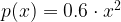
Most often than not, the intention is to reward early adopters, ensuring that the price will increase with the number of tokens sold by the market: early buyers will have cheaper prices, while those that come after will pay more. This, however, will depend on the liquidity of the market. If there is a frequent two-way movement, with frequent sales as well as purchases, the price may go down with time, as more people sell their tokens, only for it to pick up later again when the price falls below some kind of equilibrium.

Buying and selling tokens

Imagine that you want to buy a token from a TBC, and that the price function is P(S) = S / 100. If the supply is currently of 100 tokens, the price of the next full token that the curve sells will be P(100 + 1) = 1.01.

After 10 tokens are bought, the price of the next full token will rise to 1.1. If we wanted to buy 10 tokens when the supply was at 100, we’d pay 1.01 + ... + 1.10 = 10.55, for an average cost of 1.055, more or less halfway between the token price at the start and the end of our purchase.

This simple example assumes that we can only buy whole tokens, but that generally is not the case. Users are able to buy fractions of a token, and when doing so the token price will update accordingly. In the example above, if i decided to buy only 1/10th of a token the price of the first fraction would change from 1.01 to P(100 + 0.1)/10 = 0.1001. Then, for the next fraction I’d pay P(100.1 + 0.2)/10 = 0.1002, and so on until I had bought the whole first token. My total would be 0.1001 + 0.1002 + ... + 0.101 = 1.0055, which is less than the original price of 1.01. The same applies if I want to buy the next 9 tokens, bringing the total to 10.505 instead of 10.55. So, we can save money by buying smaller fractions. How small can we buy them? How do we compute the cost of buying from point A to point B in the curve?

Computing the Cost

Imagine that the user buys tokens in the smallest possible fraction.If the smallest unit we can buy is 0.001, then one unit will extend from 99.999 to 100.000, at price 1, the next will go from 100.000 to 100.001, at price 1.00001, and so on. If you draw a horizontal line for the price inside these intervals, you will have a succession of rectangles just above the price curve. The area of each rectangle represents the cost of buying each unit. If instead we paid the price of the current token (if the supply is currently 100, then you would pay 1), then we’d get rectangles under the curve, and the finer these rectangles are, the closer to the curve they would be (and the higher the cost would be). Both sets of rectangles are just approximations that follow from having some finite precision. But mathematical theory gives us the tools to consider infinite precision, when the rectangles are infinitesimally thin. In this case, the sum of their areas is exactly the area below the curve, and that quantity is given by the Integral function.

It is also the reserve of the curve at that point, since it corresponds to the total value paid to reach the current supply. That gives us a fast way to compute the cost of any trade: compute the reserve function for the supply before you trade (buy or sell) and for the supply after you trade. You pay, or receive, the difference between these two values, if the market is using the same curve for buying and selling.

The market could indeed be using different curves, which is equivalent to defining a spread. Although this is common in financial markets, it is beyond the scope of this post, so I’ll ignore that today.

The Bancor Formula

Bancor has defined a hard requirement: to maintain at all times a constant reserve ratio. It is not clear to me why they do this. As I will show below, this restricts the price functions that we can use. The function is simple and easy to understand.

The definition of reserve ratio, in mathematical terms, is this:

Reserve Ratio (RR) = Reserve (R) / (Supply (S) x Price (P))

And we are guaranteed that this ratio is constant, no matter where we are on the curve.

(From now on, I’ll use only the abbreviations to simplify.)

Using the above, we can compute the price of the next token by applying this formula:

P = R / (RR x S)

What sort of function is this? How does the price change with the supply? And how easy are these to integrate, for us to find the price of a trade?

The answer to this requires a bit of Calculus. I leave it here for those who are interested in maths, but feel free to skip it if you’d rather just take my word for it.

I’ll show you first some intuitive cases.

Constant Price

In this case, the price is always the same, and does not change with the supply. I have listed one sample point, A, at coordinates (10,10). The market cap at this point is the total supply multiplied by the price: 100. In fact, the Market Cap at one point is always defined by the rectangle whose base is the supply and the height is the price.

But the space below the curve is the exact same rectangle, given that the price is a horizontal line. Therefore, the reserve ratio must be 1, and whenever the reserve ratio is 1, the price must be a constant function.

Linear Price

In this case, we have a linear price function. For each unit that the supply increases, the price increases by two. The slope of the curve looks more or less 45º here, but that is because the axes have been scaled to different factors. The point I’m going to make is valid for any slope between 0º and 90º degrees: the area below the curve, at any point, is always a right triangle and corresponds to exactly a half of the market cap at that point. This means the reserve ratio is 1/2.

The converse is also true. If the ratio is 1/2 anywhere we must always have a linear function, but I will leave the proof for the next section.

General case

Bancor does not allow reserve ratios equal to 0. That would mean the market would never have any money to pay sellers of tokens. It also does not allow reserve ratios greater than 1. That would mean that at some point the price curve would be decreasing, and you could lose money if you sold when the supply was higher than when you bought. This is important because it limits the values we have to analyse later.

So I will now show you how we can deduce the types of functions we can have.

Let’s define some variables:

$s$ represents the supply, and is the variable of the horizontal axis
$p(s)$ represents the price for a given supply, and is plotted on the vertical axis.
$k$ is the reserve ratio

The market capitalization is, at each point, $s \cdot p(s)$ , and the reserve is given by $r(s) = \int_0^s p(x) dx$ . Because the reserve ratio is constant, the following holds for any value of $s$ :

$s \cdot p(s) \cdot k = \int_0^s p(x) dx = P(s) - P(0)$ , where $P(s)$ is the primitive (i.e., the indefinite integral) of $p(s)$ .

Derivating both sides, we get

$k \cdot (s \cdot p(s))' = P'(s)$ .

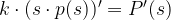
The above is a differential equation, and in general it is not always possible to solve these analytically. We are lucky, though, because this belongs to a class that can be easily solved. Here’s how to proceed.

In the above equation, the terms $P(s), P(0)$ are of different types. $0$ is a constant, and so $P(0)$ is a function with all its variables defined. Therefore, it is also a constant, and its derivative is 0. $P(s)$ , on the other hand, is a function with the free variable $s$ , the same we have on the other side of the equation. This means its derivative is also a function of $s$ and not a constant. But because $P(s)$ is the primitive of $p(s)$ , by definition $P'(s) = p(s)$ . Now, applying the rule for derivatives of multiplication on the left hand side we get:

$p(s) + s \cdot p'(s) = p(s)/k \Leftrightarrow$

$s \cdot p'(s) = \left(\frac{1}{k} - 1\right) \cdot p(s) \Leftrightarrow$

$\frac{p'(s)}{p(s)} = \left(\frac{1}{k} - 1\right) \cdot \frac{1}{s}$ .

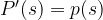
The next step involves a little creativity, necessary to recognize that on both sides of the equation we have well known derivatives:

$\frac{p'(s)}{p(s)} = [\ln p(s) + C_0]'$ , for some constant $C_0$

$\frac{1}{s} = [\ln s]'$ .

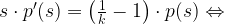
This allows us to get rid of the derivatives by integrating again:

$[\ln p(s) + C_0]' = \left(\frac{1}{k} - 1\right) \cdot [\ln s]' \Leftrightarrow$

$\ln p(s) + C_0 = \left(\frac{1}{k} - 1\right) \cdot \ln s$

To finally solve this equation and find $p(s)$ , we have only to exponentiate both sides:

$\exp (\ln p(s) + C_0) = \exp \left(\left(\frac{1}{k} - 1\right) \cdot \ln s \right) \Leftrightarrow$

$\frac{1}{C_1} \cdot p(s) = s^{\frac{1}{k} - 1} \Leftrightarrow$

$p(s) = C_1 \cdot s^{\frac{1}{k} - 1}$ .

This is the payoff, the final general expression of all the price functions accepted by Bancor.

Curve shapes

The above equation shows that a Bancor curve is completely defined by two parameters: the reserve ratio and some constant. This constant is customary when solving differential equations, and is usually defined by inputting some initial variables to the system. In the case of Bancor, that would be a legal pair in the curve, for example, “previous balance and reserve”.

The second parameter is the reserve ratio, and I find it more interesting because it sets the shape of the curve, and thereby the kind of incentives we want to promote.

Remember $0 < k \leq 1$ .

$k = 0$ : $p(s) = C \cdot s^0 = C$ –> constant function.
$k = 1/2$ : $p(s) = C \cdot s^{2-1} = C \cdot s$ –> a linear function.
$k < 1/2$ : $p(s) = C \cdot s^{z}, \mbox{ for }1 < z < +\infty$ –> a superlinear polynomial function.
$k > 1/2$ : $p(s) = C \cdot s^{z}, \mbox{ for } 0 < z < 1$ –> a sublinear polynomial function.

Following are some figures showing what these curves look like.

The first image shows three polynomial price functions, with differing exponent:

$p(x) = x^2$

$p(x) = x^{7/4}$

$p(x) = x^{5/4}$

All of these have a similar shape, and that is true of higher degree polynomials with a single term as well. The higher the exponent is, the higher the prices are in general, and the more concave the curve is, with a U-shape that becomes narrower as the exponent increases. The lower it is, the closer it is to a simple line.

This picture illustrates the exact same functions, but in the range between 0 and 1. In this interval, the behaviour of the lines is similar: lower exponents closer to a line; higher exponents more curved. But that has the effect that the lower the exponent is, the higher the price is. Lower exponents offer a smoother travel, with lower highs, but also higher lows.

The image above demonstrates three price functions, whose exponent is less than 1. The functions here are:

$p(x) = x^{3/4}$

$p(x) = x^{2/4}$

$p(x) = x^{1/4}$

These functions look a bit like a U-shape turned on its side, with a quick rise near the origin of the chart, then a gradual approximation to a horizontal line. Still, just like the polynomial functions with exponents larger than 1, these functions never have an asymptote and will not converge to any fixed straight line (horizontal or sloped).

Also, like the examples above, these functions have distinct behaviour on the different sides of $x=1$ . To the left of this line, smaller exponents rise at a quicker rate than higher exponents, but they are overtaken on the right side of this line by the higher exponents, growing much slower.

Finally, in this last picture, I show two functions with the same degree, but a different constant.

$p(x) = x^2$

$p(x) = 0.6 \cdot x^2$

They have the exact same shape, but grow at different rates because of the constant. But the point I want you to notice is that, just as predicted by the formula, the area below each curve is still exactly 1/3 of the rectangle defined by the last point of the curve. This is an empyrical demonstration of how the reserve ratio depends only on the exponent of the price function, and not on the other parameter of the curve.

That is it for today. Thank you for reading, and I hope you’ll be back another time.